Economies of scale

Economies of scale refer to the cost advantages that businesses gain as they increase their production levels. Why do these advantages occur? To understand this, let’s review some key variables and introduce new ones along with appropriate notation.
The variables discussed in the previous post
Variable Cost: \(VC(Q)\)
This is the cost that varies depending on the level of output \(Q\). In the previous post, we defined the variable cost function as:
$$VC(Q) = 0.7Q^2 + 10Q$$
Fixed Cost: \(FC\)
This is the cost that does not vary with the level of output \(Q\). In the previous post, we defined the fixed cost \(FC\) as:
$$FC = 1000$$
Total Cost: \(TC(Q) = VC(Q) + FC\)
This is the total cost, which equals the sum of variable cost and fixed cost. Therefore, our total cost function \(TC(Q)\) is
$$TC(Q) = VC(Q) + FC$$
$$=0.7Q^2 + 10Q + 1000$$
New variables
Average Variable Cost: \(AVC(Q) = VC(Q) / Q\)
This represents the variable cost per unit of output. For example, when \(Q = 10\), our \(VC(10)\) is
$$VC(Q) = 0.7Q^2 + 10Q \rightarrow$$
$$VC(10) = 0.7\times 10^2 + 10\times 10$$
$$= 170$$
So, \(AVC(10)\) is
$$AVC(Q) = VC(Q) / Q \rightarrow$$
$$AVC(10) = VC(10) / 10$$
$$= 170 / 10 = 17$$
Average Fixed Cost: \(AFC = FC / Q\)
This represents the fixed cost per unit of output. For example, when \(Q = 10\) our fixed cost \(FC = 1000\). Indeed, \(FC\) is always 1000 regardless of \(Q\), since it is fixed cost. So,
$$AVC = FC / Q$$
$$= 1000 / 10 = 100$$
Average Total Cost
$$ATC(Q) = \frac{TC(Q)}{Q}$$
$$= \frac{VC(Q)+FC}{Q} $$
This represents the total cost per unit of output. For example, at \(Q = 10\), we already calculated \(VC(10) = 170\), \(FC=1000\) So the total cost is:
$$TC(10)=VC(10) + FC$$
$$=170+1000=1170$$
Then,
$$ATC(10) = TC(10)/10$$
$$= 1170/10 =117$$
Now, we all set.
Visualizing Cost Per Unit
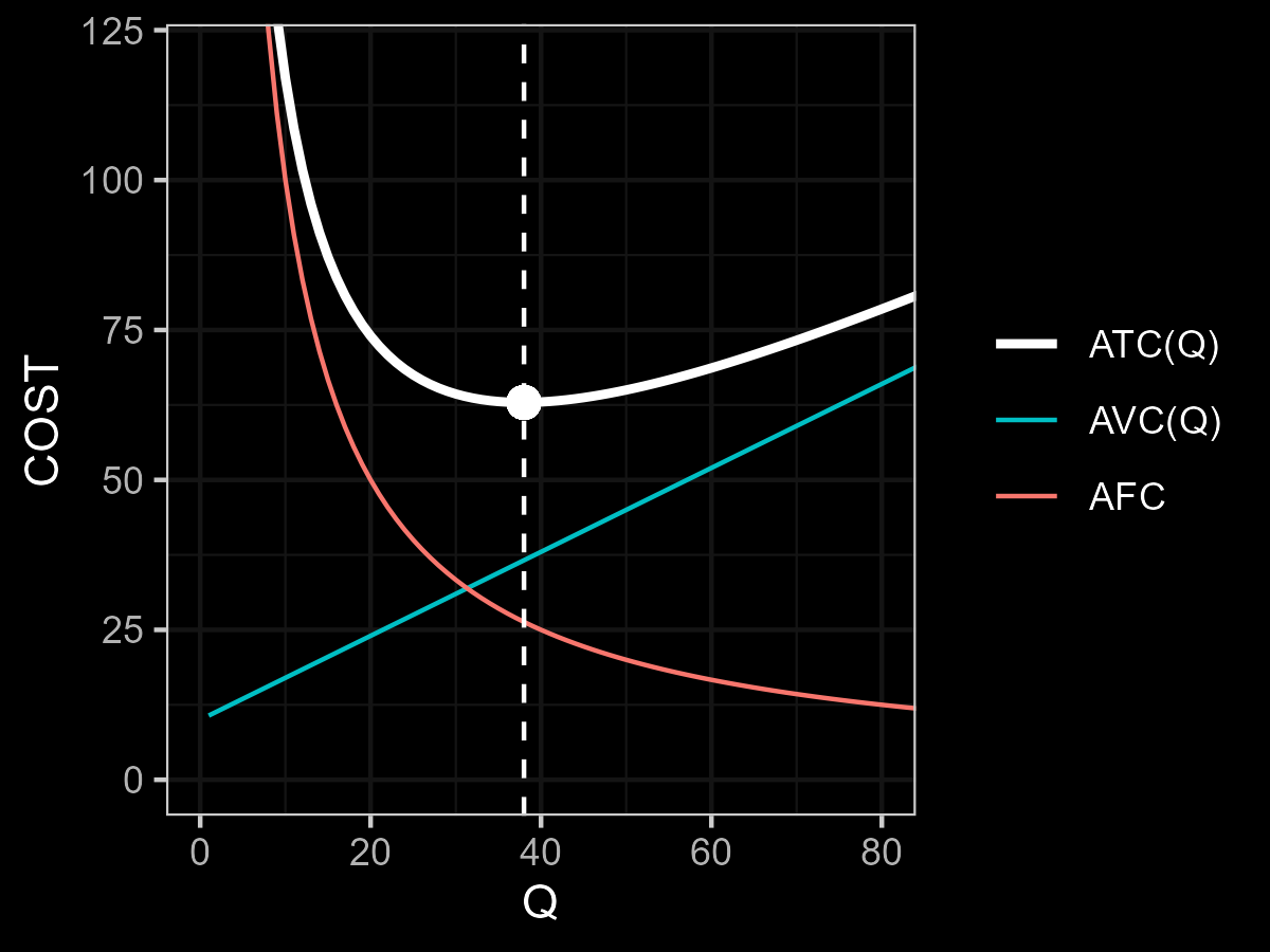
One effective way to understand cost per unit is by plotting the following cost curves:
– Average Variable Cost \(AVC(Q)\)
– Average Fixed Cost \(AFC\)
– Average Total Cost \(ATC(Q)\)
This graph will show how each component behaves as output quantity (Q) increases.

The white curve represents \(ATC(Q)\), and its minimum point marks the turning point for economies of scale.
– On the left side of this point, \(ATC(Q)\) decreases as \(Q\) increases. This is because average fixed cost (the red curve) drops sharply at first, and although \(AVC(Q)\) (the blue curve) rises, the decline in \(AFC(Q)\) offsets it.
– However, on the right side, \(ATC(Q)\) starts increasing. Why? Because the drop in \(AFC(Q)\) slows down, while the rise in \(AVC(Q)\) continues. At this stage, the increasing variable costs outweigh any remaining benefit from fixed cost spreading.
In summary:
– Economies of scale occur when increasing production leads to lower average total cost.
– But after a certain point, diseconomies of scale set in, and \(ATC(Q)\) begins to rise.
In the next post, we’ll explore how you can calculate the exact point of economies of scale using marginal cost and what kind of decision-making we can make based on this cost structure.