Finding the Best Fit: How Orthogonal Projections Simplify Linear Algebra

In our previous exploration of inner product spaces, we defined the tools for measuring “length” and “angle (orthogonality)” in abstract vector spaces. Now, it is time to put those tools to work to solve concrete problems. I will introduce the Orthogonal Decomposition Theorem. This powerful concept allows us to break any vector into a “shadow” (projection) and an “error” component. This is the mathematical foundation for finding the “best approximation” when an exact solution is impossible, bridging the gap between abstract geometry and real-world applications like curve fitting.

1. Theorem 6.5

Let $V$ be a nonzero finite-dimensional inner product space. Then $V$ has an orthonormal basis $\beta$. Furthermore, if $\beta = \{v_1, v_2, \dots, v_n\}$ and $x \in V$, then

$$
x = \sum_{i=1}^{n} \langle x, v_i \rangle v_i
$$

This theorem tells us two powerful things about finite-dimensional spaces with an inner product (like standard Euclidean space):

An “ideal” grid always exists: No matter the space, you can always find a basis where every vector has a length of 1 (normal) and is perpendicular to every other vector (orthogonal). This is called an orthonormal basis.
Coordinates are easy to find: Usually, if you want to express a vector $x$ as a combination of basis vectors, you have to solve a system of linear equations. However, if your basis is orthonormal, you can skip the hard work. The coordinate for a specific basis vector is just the inner product (dot product) of your vector $x$ with that basis vector.

Simple Example

Let’s look at the standard 2D plane ($\mathbb{R}^2$).

We have an orthonormal basis $\beta = {v_1, v_2}$ where $v_1 = (1, 0)$ and $v_2 = (0, 1)$.
We have a vector $x = (2, 5)$.

The theorem says we can find the coefficients just by doing the inner product (dot product):

Find the first coefficient: Take the dot product of $x$ and $v_1$: $$
\langle x, v_1 \rangle = (2 \cdot 1) + (5 \cdot 0) = 2
$$
Find the second coefficient: Take the dot product of $x$ and $v_2$: $$
\langle x, v_2 \rangle = (2 \cdot 0) + (5 \cdot 1) = 5
$$
Build the vector: $$
x = 2v_1 + 5v_2
$$

This confirms the theorem: the inner products ($2$ and $5$) gave us the exact coordinates needed to build $x$.

2. Corollary to Theorem 6.5

Let $V$ be a finite-dimensional inner product space with an orthonormal basis $\beta = \{v_1, v_2, \dots, v_n\}$. Let $T$ be a linear operator on $V$, and let $A = [T]_\beta$. Then for any $i$ and $j$:

$$
A_{ij} = \langle T(v_j), v_i \rangle
$$

This corollary builds directly on the previous theorem to help us build matrices for linear transformations very easily.

Normally, to find the matrix entry $A_{ij}$ (the number in row $i$, column $j$), you have to:

Apply the transformation $T$ to the $j$-th basis vector ($v_j$).
Take the result and figure out how to write it as a combination of all basis vectors.
Extract the coefficient for $v_i$.

That step 2 is usually tedious algebra. However, because the basis is orthonormal, this corollary says you can find that specific entry just by taking the inner product of the transformed vector $T(v_j)$ and the basis vector $v_i$. No algebra required!

Simple Example

Let’s work in $\mathbb{R}^2$ with the standard orthonormal basis $v_1 = (1, 0)$ and $v_2 = (0, 1)$.

Let the transformation $T$ be defined by $T(x, y) = (2x + y, \ x – 3y)$. We want to find the matrix entry $A_{21}$ (Row 2, Column 1).

Identify $j$ and $i$: Since we want $A_{21}$, we are looking at Column $j=1$ and Row $i=2$. The formula says: $A_{21} = \langle T(v_1), v_2 \rangle$.
Compute $T(v_1)$: $$
T(v_1) = T(1, 0) = (2(1)+0, \ 1-3(0)) = (2, 1)
$$
Compute the Inner Product: $$
A_{21} = \langle (2, 1), v_2 \rangle = \langle (2, 1), (0, 1) \rangle
$$ $$
A_{21} = (2 \cdot 0) + (1 \cdot 1) = 1
$$

So the entry in the bottom-left corner of the matrix is 1.

3. Definition: Orthogonal Complement

Let $S$ be a nonempty subset of an inner product space $V$. We define $S^\perp$ (read “$S$ perp”) to be the set of all vectors in $V$ that are orthogonal to every vector in $S$; that is:

$$
S^\perp = {x \in V : \langle x, y \rangle = 0 \text{ for all } y \in S}
$$

The set $S^\perp$ is called the orthogonal complement of $S$.

While we often visualize “orthogonal” as being perpendicular (90 degrees) in physical space, the mathematical definition is much broader. In linear algebra, two vectors are orthogonal solely if their inner product is zero:

$$
\langle x, y \rangle = 0
$$

The “orthogonal complement” ($S^\perp$) collects every single vector $x$ that satisfies this condition for all $y$ in your set $S$. This definition works even for abstract spaces where you cannot “see” an angle—like spaces of polynomials or continuous functions.

Simple Example

Let’s look at two different contexts to see how this works.

1. Standard Geometry ($\mathbb{R}^3$):

If $S$ is the $z$-axis (vectors like $(0,0,1)$), then $S^\perp$ is the entire $xy$-plane. Any vector on the floor $(x, y, 0)$ has a zero dot product with any vector on the vertical axis.

$$
\langle (0,0,1), (x,y,0) \rangle = 0 + 0 + 0 = 0
$$

2. Abstract Space (Polynomials)

To understand orthogonality beyond geometry, we need to define our “world” (the vector space) and our “ruler” (the inner product).

The Setup:

Vector Space ($V$): Let $V$ be the vector space of all real-valued polynomials defined on the interval $[0, 1]$.
Inner Product: We define the inner product for any two polynomials $f(t)$ and $g(t)$ in this space as the integral of their product: $$
\langle f, g \rangle = \int_{0}^{1} f(t)g(t) \, dt
$$

The Example:

Let our set $S$ contain just the constant function:

$$
f(t) = 1
$$

We want to find a vector in the orthogonal complement $S^\perp$. Consider the function:

$$
g(t) = 2t – 1
$$

Visually, $f(t)$ is a flat horizontal line and $g(t)$ is a slanted line crossing the axis. They do not look perpendicular in a geometric sense. However, let’s check if they are orthogonal using our definition:

$$
\langle f, g \rangle = \int_{0}^{1} (1) \cdot (2t – 1) \, dt
$$

$$
= \left[ t^2 – t \right]_{0}^{1}
$$

$$
= (1^2 – 1) – (0^2 – 0) = 0
$$

Conclusion:

Since the integral is zero, $\langle f, g \rangle = 0$. Therefore, $g(t)$ lives in the orthogonal complement of $f(t)$, even though they are just functions!

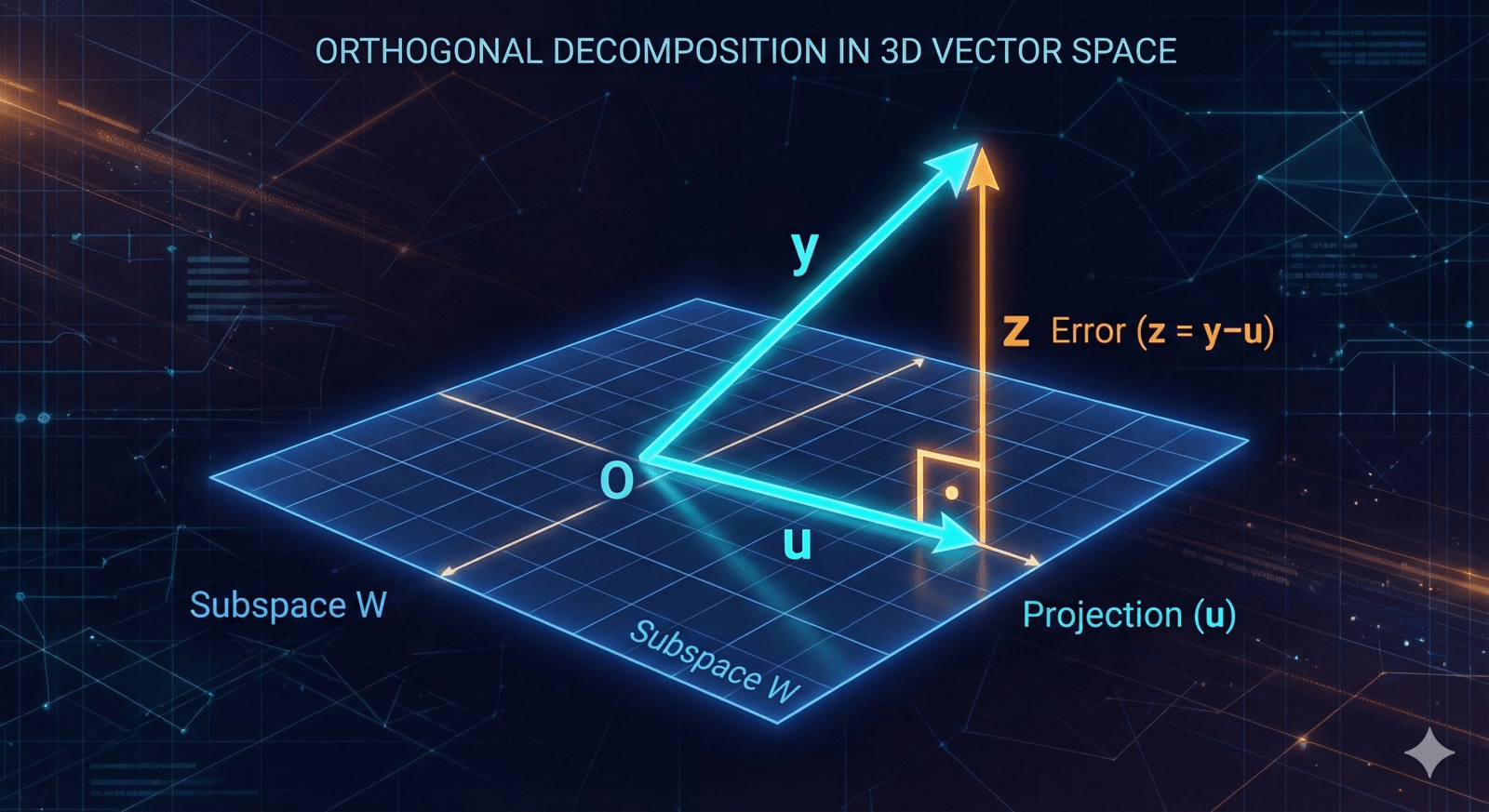
4. Theorem 6.6: Orthogonal Decomposition

Let $W$ be a finite-dimensional subspace of an inner product space $V$, and let $y \in V$. Then there exist unique vectors $u \in W$ and $z \in W^\perp$ such that $y = u + z$. Furthermore, if ${v_1, v_2, \dots, v_k}$ is an orthonormal basis for $W$, then

$$
u = \sum_{i=1}^{k} \langle y, v_i \rangle v_i
$$

This theorem is about decomposition. It says that any vector $y$ in a big space $V$ can be split cleanly into two distinct parts relative to a subspace $W$:

The “Shadow” ($u$): This part lives entirely inside the subspace $W$. This vector $u$ is the “best approximation” of $y$ that exists within $W$. It is often called the orthogonal projection of $y$ onto $W$.
The “Error” ($z$): This part is completely orthogonal to $W$ (it lives in $W^\perp$). It represents the “height” or distance perpendicular to the subspace.

Most importantly, this split is unique. There is only one way to break $y$ down like this.

Simple Example

Let’s go back to our 3D space ($\mathbb{R}^3$) and our flat floor.

The Space: Let $V = \mathbb{R}^3$.
The Subspace ($W$): Let $W$ be the $xy$-plane.
- An orthonormal basis for $W$ is $v_1 = (1, 0, 0)$ and $v_2 = (0, 1, 0)$.
The Vector ($y$): Let $y = (3, 4, 9)$.

Goal: Split $y$ into a part in the plane ($u$) and a part perpendicular to the plane ($z$).

Calculate $u$ (The Projection): Using the formula from the theorem: $$
u = \langle y, v_1 \rangle v_1 + \langle y, v_2 \rangle v_2
$$ $$
u = (3 \cdot 1 + 4 \cdot 0 + 9 \cdot 0)v_1 + (3 \cdot 0 + 4 \cdot 1 + 9 \cdot 0)v_2
$$ $$
u = 3(1, 0, 0) + 4(0, 1, 0) = (3, 4, 0)
$$ Notice: This is just the “shadow” of the vector on the floor.
Calculate $z$ (The Perpendicular Component): Since $y = u + z$, we know $z = y – u$. $$
z = (3, 4, 9) – (3, 4, 0) = (0, 0, 9)
$$
Check:
- Does $u$ live in the $xy$-plane ($W$)? Yes.
- Is $z$ perpendicular to the $xy$-plane ($W^\perp$)? Yes (it points straight up).
- Do they add up to $y$? $(3, 4, 0) + (0, 0, 9) = (3, 4, 9)$. Yes.

Here is the breakdown for the Corollary to Theorem 6.6. This is often called the “Best Approximation Theorem.”

5. Corollary to Theorem 6.6

In the notation of Theorem 6.6, the vector $u$ is the unique vector in $W$ that is “closest” to $y$; that is, for any $x \in W$,

$$
||y – x|| \geq ||y – u||
$$

and this inequality is an equality if and only if $x = u$.

This corollary answers a very practical question: “If I can’t reach the exact vector $y$ because I am stuck inside the subspace $W$, what is the single best substitute I can use?”

The answer is the orthogonal projection $u$.

Geometrically, this is intuitive. Imagine you are standing in a room ($W$, the floor) and there is a light bulb hanging from the ceiling ($y$). If you want to stand on the floor exactly where you are closest to the bulb, you stand directly underneath it. That spot is $u$. If you move to any other spot $x$ on the floor, you are moving away from the bulb, increasing the distance.

Simple Example

Let’s reuse our previous setup to prove this with numbers.

The Vector ($y$): $y = (3, 4, 9)$
The Subspace ($W$): The $xy$-plane (all vectors where $z=0$).
The Projection ($u$): As calculated before, $u = (3, 4, 0)$.

Let’s compare the distance from $y$ to $u$ versus the distance from $y$ to some random other point $x$ in the subspace.

Distance to the Projection ($u$): $$
y – u = (0, 0, 9)
$$ $$
\text{Distance} = ||y – u|| = 9
$$
Distance to a Random Point ($x$): Let’s pick a different point on the floor, say $x = (5, 2, 0)$. $$
y – x = (3-5, 4-2, 9-0) = (-2, 2, 9)
$$ $$
\text{Distance} = ||y – x|| = \sqrt{(-2)^2 + 2^2 + 9^2}
$$ $$
= \sqrt{4 + 4 + 81} = \sqrt{89} \approx 9.43
$$

Conclusion:

Since $9 < 9.43$, the projection $u$ is indeed closer to $y$ than $x$ is. No matter what other $x$ you pick, the distance will always be greater than 9.

The vector u in the corollary is called the orthogonal projection of y on W.

6. Theorem 6.7: Extension and Dimension

Suppose that $S = \{v_1, v_2, \dots, v_k\}$ is an orthonormal set in an $n$-dimensional inner product space $V$. Then

(a) $S$ can be extended to an orthonormal basis ${v_1, v_2, \dots, v_k, v_{k+1}, \dots, v_n}$ for $V$.

(b) If $W = \text{span}(S)$, then $S_1 = \{v_{k+1}, v_{k+2}, \dots, v_n\}$ is an orthonormal basis for $W^\perp$ (using the preceding notation).

This theorem gives us a complete “roadmap” for building bases in vector spaces:

You can always finish what you started (Part a): If you have a few vectors that are orthonormal (length 1 and perpendicular to each other), you are never “stuck.” You can always find more vectors to complete the set until you have a full basis for the entire space.
The “New” vectors define the Complement (Part b): When you add those new vectors to finish the basis, you haven’t just added random vectors. Those specific new vectors form a perfect basis for the orthogonal complement ($W^\perp$).
The Dimensions add up (Part c): This is a simple counting rule. The size of the subspace ($W$) plus the size of its perpendicular part ($W^\perp$) equals the size of the whole space ($V$).

Simple Example

Let’s work in 3D space ($V = \mathbb{R}^3$), so the total dimension is $n=3$.

Start with an orthonormal set ($S$): Let $S = {v_1}$ where $v_1 = (1, 0, 0)$. This defines our subspace $W$ (the x-axis). $\dim(W) = 1$.
Extend it (Part a): We need to fill out the space. We can add $v_2 = (0, 1, 0)$ and $v_3 = (0, 0, 1)$. Now we have a full orthonormal basis for $\mathbb{R}^3$: ${(1,0,0), (0,1,0), (0,0,1)}$.
Identify the Complement (Part b): The vectors we added were $S_1 = {v_2, v_3}$. These two vectors span the $yz$-plane. The $yz$-plane is exactly perpendicular to the x-axis. So, $S_1$ is indeed the basis for $W^\perp$.
Check Dimensions (Part c): $\dim(V) = 3$ (The whole space) $\dim(W) = 1$ (The x-axis) $\dim(W^\perp) = 2$ (The yz-plane) $$
3 = 1 + 2
$$ The math holds up perfectly!

The integrated example: Approximating a Parabola with a Straight Line

Let’s wrap up this post with an integrated example.

The Setup:

Vector Space ($V$): Let $V = P_2(\mathbb{R})$, the space of polynomials of degree at most 2.
Inner Product: We will use the standard integral inner product on the interval $[0, 1]$: $$
\langle f, g \rangle = \int_0^1 f(t)g(t) \, dt
$$
Subspace ($W$): Let $W = P_1(\mathbb{R})$, the subspace of linear polynomials (straight lines of the form $at+b$).
Target Vector ($y$): Let $y = t^2$. We want to “project” this parabola onto the space of straight lines $W$.

Step 1: Finding an Orthonormal Basis for $W$

To use Theorem 6.6, we first need an orthonormal basis ${u_1, u_2}$ for our subspace $W$ (lines).

Starting with the standard basis ${1, t}$, we apply the Gram-Schmidt process on $[0, 1]$:

First vector ($u_1$): Normalize $v_1 = 1$. Since $\int_0^1 1^2 dt = 1$, we have: $$
u_1(t) = 1
$$
Second vector ($u_2$): Take $v_2 = t$ and subtract its projection onto $u_1$: $$
\text{orthogonal part} = t – \langle t, u_1 \rangle u_1
$$ $$
= t – \left(\int_0^1 t \cdot 1 \, dt\right) \cdot 1 = t – \frac{1}{2}
$$ Now, normalize $t – 1/2$. The squared norm is $\int_0^1 (t – 1/2)^2 dt = \frac{1}{12}$. Dividing by the norm ($1/\sqrt{12}$), we get: $$
u_2(t) = \sqrt{12}(t – 1/2) = \sqrt{3}(2t – 1)
$$

Basis: ${u_1, u_2} = {1, \sqrt{3}(2t-1)}$ is our orthonormal basis for $W$.

Step 2: Applying Theorem 6.6 (The Projection)

According to the theorem, the projection $u$ is the sum of the components of $y$ along the basis vectors:

$$
u = \langle y, u_1 \rangle u_1 + \langle y, u_2 \rangle u_2
$$

Let’s calculate the inner products (Fourier coefficients):

First Coefficient: $$
\langle t^2, u_1 \rangle = \int_0^1 t^2 \cdot 1 \, dt = \left[\frac{t^3}{3}\right]_0^1 = \frac{1}{3}
$$
Second Coefficient: $$
\langle t^2, u_2 \rangle = \int_0^1 t^2 \cdot \sqrt{3}(2t-1) \, dt = \sqrt{3} \int_0^1 (2t^3 – t^2) \, dt
$$ $$
= \sqrt{3} \left( \frac{2}{4} – \frac{1}{3} \right) = \sqrt{3} \left( \frac{1}{2} – \frac{1}{3} \right) = \frac{\sqrt{3}}{6}
$$

Now, construct $u$:

$$
u(t) = \left(\frac{1}{3}\right)(1) + \left(\frac{\sqrt{3}}{6}\right)\sqrt{3}(2t-1)
$$

$$
u(t) = \frac{1}{3} + \frac{3}{6}(2t-1) = \frac{1}{3} + t – \frac{1}{2}
$$

$$
u(t) = t – \frac{1}{6}
$$

Result: The orthogonal projection of $t^2$ onto the subspace of lines is $u(t) = t – \frac{1}{6}$.

Step 3: Understanding “Orthogonality”

Theorem 6.6 states that $y = u + z$, where $u \in W$ and $z \in W^{\perp}$.

Here, our “error vector” is $z = y – u = t^2 – (t – 1/6)$.

What does it mean for $z$ to be orthogonal to $W$?

You might worry that the curve $t^2$ and the line $t – 1/6$ do not look like they are at a “90-degree angle” visually. You are correct—in function spaces, geometry is a metaphor.

Instead of lines crossing at 90 degrees, “orthogonality” is defined purely by the inner product being zero: $\langle z, w \rangle = 0$.

$$
\langle z, w \rangle = \int_0^1 z(t)w(t) \, dt = 0
$$

Let’s verify this “abstract 90-degree” relationship. If $z$ is truly orthogonal to the subspace $W$ (lines), it must be orthogonal to the basis vector $1$:

$$
\langle z, 1 \rangle = \int_0^1 \left(t^2 – t + \frac{1}{6}\right) \cdot 1 \, dt
$$

$$
= \left[ \frac{t^3}{3} – \frac{t^2}{2} + \frac{t}{6} \right]_0^1 = \frac{1}{3} – \frac{1}{2} + \frac{1}{6}
$$

$$
= \frac{2}{6} – \frac{3}{6} + \frac{1}{6} = 0
$$

Step 4: Applying the Corollary (Best Approximation)

The corollary states that $u = t – 1/6$ is the “closest” vector to $y=t^2$.

In the context of polynomials, “closest” means it minimizes the “energy” of the error:

$$
|| y – x ||^2 = \int_0^1 (t^2 – (at+b))^2 \, dt
$$

Any other line $x(t) = at+b$ you try to draw will result in a larger integral result than the line $t – 1/6$.

References

The theorem numbering in this post follows Linear Algebra (4th Edition) by Friedberg, Insel, and Spence. Some explanations and details here differ from the book.

Finding the Best Fit: How Orthogonal Projections Simplify Linear Algebra

1. Theorem 6.5

2. Corollary to Theorem 6.5

3. Definition: Orthogonal Complement

4. Theorem 6.6: Orthogonal Decomposition

5. Corollary to Theorem 6.6

6. Theorem 6.7: Extension and Dimension

The integrated example: Approximating a Parabola with a Straight Line

Step 1: Finding an Orthonormal Basis for \(W\)

Step 2: Applying Theorem 6.6 (The Projection)

Step 3: Understanding “Orthogonality”

Step 4: Applying the Corollary (Best Approximation)

References

Leave a ReplyCancel Reply