A Linear Algebra Approach to Least Squares

In science and engineering, we rarely get perfect data. When we collect measurements $(t_i, y_i)$, they almost never fall perfectly on a straight line due to noise or experimental error. We are usually looking for the “best fit” line $y = ct + d$ to describe the trend. But what does “best fit” or “least squares” actually mean mathematically?

While this is often taught as a calculus problem (minimizing the sum of squared errors), it is actually a beautiful problem in Linear Algebra. It is a story about geometry, projections, and subspaces.

1. From Statistics to Linear Algebra

Let’s say we have $m$ data points. We are trying to solve a system of linear equations that looks like this:

$$
\begin{cases} ct_1 + d = y_1 \\ ct_2 + d = y_2 \\ \vdots \\ ct_m + d = y_m \end{cases}
$$

In matrix notation, we define our Design Matrix $A$, our Unknowns $x$, and our Observations $y$:

$$
A = \begin{pmatrix} t_1 & 1 \\ \vdots & \vdots \\ t_m & 1 \end{pmatrix}, \quad x = \begin{pmatrix} c \\ d \end{pmatrix}, \quad y = \begin{pmatrix} y_1 \\ \vdots \\ y_m \end{pmatrix}
$$

We want to solve $Ax = y$. However, because of the noise, $y$ is not in the column space of $A$ (denoted as $\mathsf{W}$).

Instead of a perfect solution, we seek a vector $x$ that minimizes the “error” $E$. In Linear Algebra, this error is the square of the norm of the residual vector:

$$
E = || y – Ax ||^2
$$

Why $E = || y – Ax ||^2$?

To understand this notation, we have to look at the error for each individual data point.

1. The Individual Error

For a single data point $(t_i, y_i)$, our line predicts the value $ct_i + d$. The difference between the actual observed value ($y_i$) and the predicted value is the error for that specific point:

$$
e_i = y_i – (ct_i + d)
$$

2. The Error Vector

In matrix notation, $Ax$ represents the vector of all our predicted values:

$$
Ax = \begin{pmatrix} ct_1 + d \\ \vdots \\ ct_m + d \end{pmatrix} = \text{Predicted Values}
$$

If we subtract this prediction vector from our observation vector $y$, we get a single vector $e$ containing all the individual errors:

$$
e = y – Ax = \begin{pmatrix} y_1 – (ct_1 + d) \\ \vdots \\ y_m – (ct_m + d) \end{pmatrix} = \begin{pmatrix} e_1 \\ \vdots \\ e_m \end{pmatrix}
$$

3. The Squared Norm

In statistics, we want to minimize the Sum of Squared Errors (SSE) to avoid negative errors canceling out positive ones. Mathematically, this is:

$$
\text{SSE} = \sum_{i=1}^{m} e_i^2 = e_1^2 + e_2^2 + \dots + e_m^2
$$

In Linear Algebra, the length (or magnitude) of a vector $v$ is called its Norm, denoted as $||v||$. If we use the standard inner product here, the formula for the norm is the square root of the sum of squared components:

$$
||e|| = ||y-Ax|| = \sqrt{e_1^2 + e_2^2 + \dots + e_m^2}
$$

If we square both sides to get rid of the square root, we get exactly the Sum of Squared Errors:

$$
||e||^2 = ||y-Ax||^2 = e_1^2 + e_2^2 + \dots + e_m^2 = \text{SSE}
$$

Therefore, minimizing the sum of squared errors is mathematically identical to minimizing the squared length of the error vector:

$$
E = || \underbrace{y – Ax}_{\text{error vector}} ||^2
$$

Because the norm is always non-negative ($||v|| \ge 0$), finding an $x$ that minimizes $||y-Ax||^2$ is equivalent to finding an $x$ that minimizes $||y-Ax||$. Thus, the problem translates simply to: Find $x$ such that the vector $Ax$ is as close as possible to $y$.

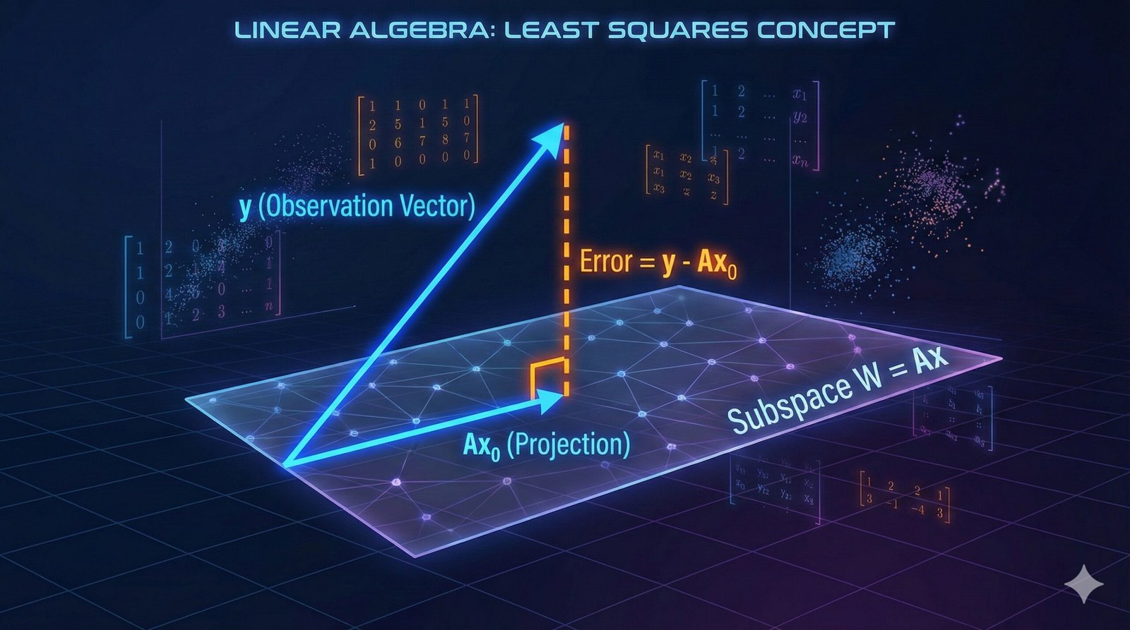
2. The Solution: Geometry of Projections

To solve this, we rely on subspaces.

Theorem 6.6: Orthogonal Decomposition

This theorem tells us that any vector $y$ can be split uniquely into two perpendicular components relative to a subspace $\mathsf{W}$.

Let $\mathsf{W}$ be a finite-dimensional subspace of an inner product space $\mathsf{V}$, and let $y \in \mathsf{V}$. Then there exist unique vectors $u \in \mathsf{W}$ and $z \in \mathsf{W}^{\perp}$ such that $y = u + z$.

Connecting to Our Least Squares Problem:

To see why this theorem is the key, we map its notation to our problem:

The Subspace ($\mathsf{W}$): This matches the Column Space (Range) of our matrix $A$, defined as $\{Ax : x \in \mathsf{F}^n\}$.
The Vector ($u$): This matches our ideal approximation $Ax_0$. It is the “shadow” or projection of $y$ onto the subspace $\mathsf{W}$.
The Vector ($z$): This matches our error vector $y – Ax_0$. This represents the “noise” that is orthogonal to our model.

Corollary: The Closest Vector

The corollary to Theorem 6.6 gives us our optimization criterion.

The vector $u$ is the unique vector in $\mathsf{W}$ that is “closest” to $y$; that is, $||y – x|| \geq ||y – u||$ for all $x \in \mathsf{W}$.

In our context, this confirms that if we can find the $x_0$ that makes the error vector ($y – Ax_0$) orthogonal to the column space, we have mathematically guaranteed the minimum error.

3. The Algebraic Tools

To find the actual values for $x$, we need two algebraic lemmas to manipulate our equations.

Lemma 1: The Adjoint Property

This allows us to move the matrix $A$ from one side of an inner product to the other.

$\langle Ax, y \rangle_m = \langle x, A^*y \rangle_n$

Lemma 2: Rank Preservation

This ensures that our solution will be unique.

If $\text{rank}(A) = n$, then $\text{rank}(A^A) = n$. Consequently, $A^A$ is invertible.

If $\text{rank}(A) = n$, then $\text{rank}(A^*A) = n$. Consequently, $A^*A$ is invertible.

4. The Solution: Deriving the Normal Equations

We now combine the geometry (Theorem 6.6) with the algebra (Lemma 1) to solve for $x_0$.

Step 1: The Orthogonality Condition

From Theorem 6.6, we established that the optimal error vector ($Ax_0 – y$) must be in $\mathsf{W}^\perp$. This means it must be orthogonal to every vector in the column space $\mathsf{W}$.

Since every vector in $\mathsf{W}$ can be written as $Ax$ for some $x$, we can write this condition as an inner product:

$$
\langle Ax, Ax_0 – y \rangle_m = 0 \quad \text{for all } x \in \mathsf{F}^n
$$

Step 2: Moving the Matrix (Lemma 1)

We want to isolate $x$, so we use Lemma 1 to move $A$ from the left side of the inner product to the right side (where it becomes the adjoint $A^*$):

$$
\langle x, A^*(Ax_0 – y) \rangle_n = 0 \quad \text{for all } x \in \mathsf{F}^n
$$

Step 3: Solving for Zero

If the inner product of a vector $v$ with any vector $x$ is always 0, then $v$ itself must be the zero vector. Therefore:

$$
A^*(Ax_0 – y) = 0
$$

Expanding this gives us:

$$
A^Ax_0 – A^y = 0 \Rightarrow A^Ax_0 = A^y
$$

Step 4: Invertibility (Lemma 2)

Finally, if we assume our data columns are linearly independent (rank($A$) = $n$), Lemma 2 tells us that $A^*A$ is invertible. We can multiply by the inverse to isolate $x_0$.

This leads to Theorem 6.12:

Let $A$ be an $m \times n$ matrix with rank $n$. The unique vector $x_0$ that minimizes $||Ax – y||$ is given by:

$$
x_0 = (A^A)^{-1}A^y
$$

These are the famous Normal Equations.

5. A Numerical Deep Dive

Let’s apply this theorem to a concrete data set to verify the geometry explicitly.

The Data:

$$
\begin{array}{c|c} t \text{ (Independent)} & y \text{ (Dependent)} \\ \hline 1 & 1.04 \\ 2 & 3.54 \\ 3 & 4.31 \\ 4 & 7.81 \\ 5 & 9.29 \\ 6 & 11.94 \\ \end{array}
$$

Step 1: Construct the Matrices

$$
A = \begin{pmatrix} 1 & 1 \\ 2 & 1 \\ 3 & 1 \\ 4 & 1 \\ 5 & 1 \\ 6 & 1 \end{pmatrix}, \quad y = \begin{pmatrix} 1.04 \\ 3.54 \\ 4.31 \\ 7.81 \\ 9.29 \\ 11.94 \end{pmatrix}
$$

Step 2: Solve for $x$ (The Coefficients)

Using the formula $x = (A^T A)^{-1} A^T y$, we calculate:

$$
\beta_1 \approx 2.164, \quad \beta_0 \approx -1.250
$$

So our best fit line is $y = 2.164t – 1.250$.

6. Verifying the Geometry (Theorem 6.6)

Here is where it gets interesting. We claimed that the data $y$ splits into a signal $u$ and noise $z$. Let’s calculate them.

The Signal Vector $u$ (in $\mathsf{W}$)

$$
u = Ax \approx \begin{pmatrix} 0.91 \\ 3.08 \\ 5.24 \\ 7.41 \\ 9.57 \\ 11.74 \end{pmatrix}
$$

Dimension: $\mathsf{W}$ is 2-dimensional.
Basis of $u$: The vector $u$ is formed by a linear combination of the two columns of A.

The Noise Vector $z$ (in $\mathsf{W}^{\perp}$)

$$
z = y – u \approx \begin{pmatrix} 0.13 \\ 0.46 \\ -0.93 \\ 0.40 \\ -0.28 \\ 0.20 \end{pmatrix}
$$

Does $z$ really live in $\mathsf{W}^{\perp}$?

For $z$ to be in $\mathsf{W}^{\perp}$, it must be orthogonal to the columns of $A$.

$$
z \cdot \text{Column}_1(A) \approx 0
$$

$$
z \cdot \text{Column}_2(A) \approx 0
$$

Numerical checks confirm these are effectively zero ($< 10^{-14}$). Theorem 6.6 holds!

The Dimensionality of Error

It is worth noting the dimensions here.

Our total space $\mathsf{V}$ is 6-dimensional (6 data points).
Our model space $\mathsf{W}$ is 2-dimensional (slope and intercept).
Therefore, our error space $\mathsf{W}^{\perp}$ is 4-dimensional ($6-2=4$).

The vector $z$ is not random; it lives in a specific 4-dimensional subspace defined by the null space of $A^T$. We can even find a basis for this error space (4 vectors orthogonal to $A$) and express $z$ as a unique combination of those basis vectors.

Conclusion

Least Squares is not just a formula to memorize. It is a projection. We project our messy, high-dimensional data $y$ onto the clean, lower-dimensional subspace $\mathsf{W}$ to find the shadow $u$ that best represents reality.

References

The theorem numbering in this post follows Linear Algebra (4th Edition) by Friedberg, Insel, and Spence. Some explanations and details here differ from the book.